By this point in time, there’s no need to emphasize how important deep learning has become. Yet, despite paving the way for some of the boldest and most complicated projects of this decade, much of deep learning’s theoretical guarantees remain unexplained.

According to classical statistical learning theory, the structure displayed by deep networks entails poor predictions over unseen instances. However, this is not often the case and, this mismatch between theory and practice is what gives deep learning a sort of magical appearance. Meanwhile, this aura is besieged by researchers that will try to tap into what really allows these models to perform so well.

To discuss this issue more closely, we need to formulate its setting. In classification problems, we typically have:

• A candidate model (or hypothesis) $h$ that maps the domain $x$ to the output $y$;
• A set of $n$ coupled observations $\mathcal{S_n} = \{ (x_1;y_1), …, (x_n; y_n) \}$, sampled from an unknown probability distribution $\mathcal{D}$;
• A target function $f$ that determines the output $y \in \{-1;1\}$ depending on the input $x$;
• A loss function $\ell$ that measures the prediction error of $h$ with respect to $f$.

In this setting, we would like to find a model that most closely approximates the target function $f$. According to our sampling distribution, this entails minimizing our expected risk: the the expected value of the error with respect to our $\mathcal{D}$:

$$R(h) := \mathbb{E}_{\mathcal{D}}[\ell(h, f)] \equiv \int_{\mathcal{X}} \ell(h(x), f(x))\,p(x)dx$$

We generate these candidates through a learning algorithm $\mathcal{A}$, that given a set of observations outputs a hypothesis. Knowing that we cannot access the sampling probability, our compass in this search is our training set. In other words, our proxy for the expected risk is the empirical risk: $$R_n(h) := \sum_{i=1}^n \ell(h(x_i), y_i).$$

Using the principle of Empirical Risk Minimization (ERM), we are assuming that the solution that minimizes the empirical risk also minimizes the expected risk. We say that a learning algorithm generalizes if the empirical risk approaches the expected risk as data grows to infinity. In other words, the generalization error, $\Delta R = R(h)-R_n(h)$ goes to zero. On the other hand, when this difference remains significantly large, we say the model overfits.

But consider the following, if we could access every conceivable hypothesis, what guarantee could ERM provide of finding a candidate that does not overfit? Think of the hypothesis that memorizes all training points and output their correct classification. Under ERM, we’d be finding a good candidate, since it perfectly fits our training data. However, when predicting an unseen observation, this model would be no better them random guessing, thus generalizing poorly.

To circumvent this, we limit our search space to a certain class of hypotheses, by only considering models with a certain structure (e.g. linear predictors). Here we essentially apply a set of assumptions of our model based on some prior knowledge of the problem, what we call inductive bias.

Under these circumstances, ERM is guaranteed to generalize as the number of data points grows to infinity. But more importantly, if our training data is sampled iid, we can devise bounds that indicate, with a small probability of error $\delta$, how close we are from the true risk.

$$\underset{S\sim\mathcal{D}^N}{\mathbb{P}}\left(R(h) - R_n(h) \le O\left (\frac{C(\mathcal{H})}{\sqrt{n}} \right)\right) > 1- \delta$$

These bounds are naturally governed by the number of data points, but also by the complexity $C$ of our hypothesis class. When considering finite sets of hypotheses, the complexity measure can simply be represented by the cardinality of the set. However, under infinte hypothesis classes, more elaborated techniques are needed.

Many competing complexity measures, and consequently generalization bounds, have been developed over the last 30 years: VC-dimension, Rademacher complexity, covering numbers, and so on. If we think about the effect of complexity on the generalization gap, the more complex a class is, the bigger the generalization gap can be. Even with a large amount of data, if the complexity measure of the model is too high, we have fewer guarantees of avoiding overfitting.

For the sake of illustration, let’s take the number of parameters of a neural network as a measure of its complexity. The MNIST dataset consists of images of handwritten digits in a 28x28 grid and contains more than 55 thousand data points. A fairly simple model, as an off-the-shelf LeNet contains more than 470 thousand parameters only in its first layer, let alone in the rest of the network. Due to its complexity, for this model to generalize with an acceptable error and probability, we would need trillions and trillions of data points. If we took this model and train it over MNIST, our natural inclination would be to think that a great performance in a training set would be the result of an interpolation of the data points, due to the large overparametrization of the model when compared to the dataset.

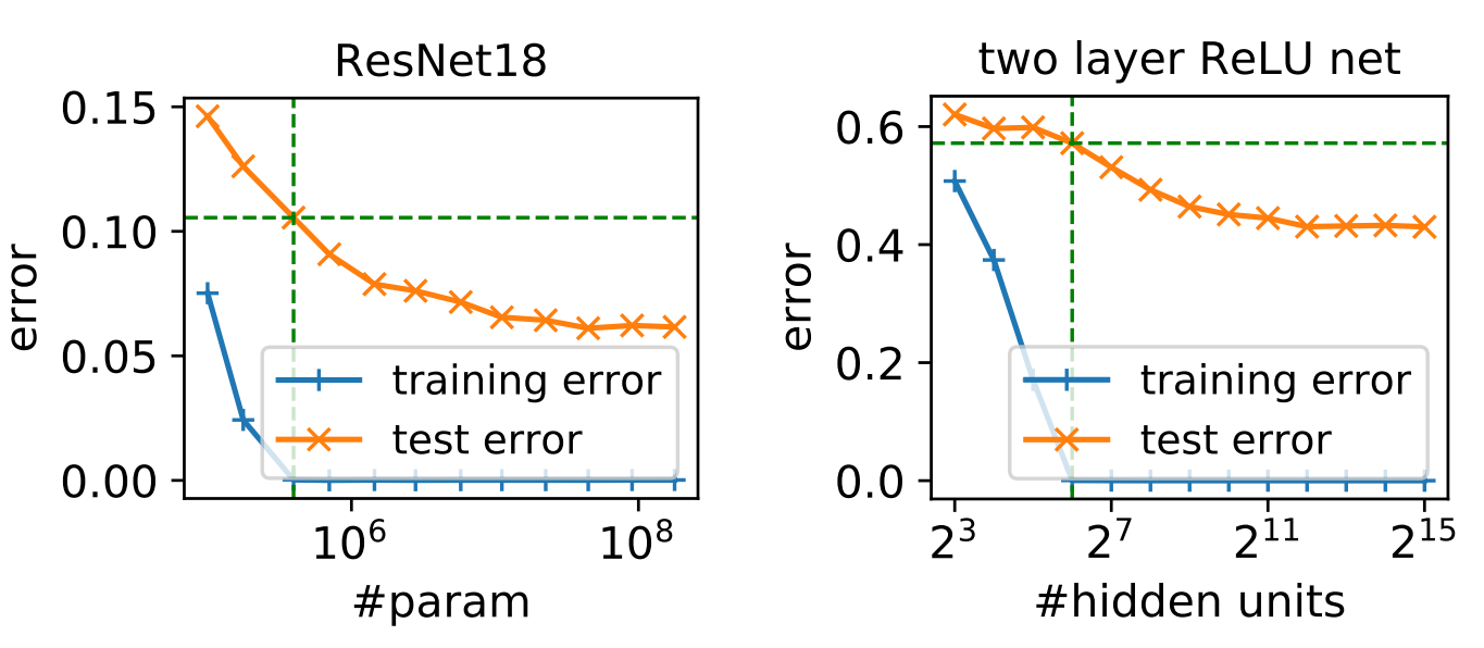
Still, we have tons of evidence that support generalization of under these settings. So… what gives?

Structured Risk Minimization and Regularization

By observing the bounds generated over the complexity of neural networks, we may think that without tremendous amounts of data, we cannot achieve generalization. However, imagine we had a class of hypothesis with a hierarchical structure, i.e. $\mathcal{H} \supseteq \mathcal{H}_1 … \supseteq \mathcal{H}_n$. In this class, each subset $\mathcal{H_i}$ has a smaller complexity than its supersets $C(\mathcal{H}) \ge C(\mathcal{H}_1) … \ge C(\mathcal{H}_n)$. If we could exploit the hierarchical structure, we can devise a way to learn a function while also minimizing its complexity, thus generating reasonable bounds. Akin to the ERM, this principle is called Structured Risk Minimization (SRM). However, if we even encounter such hierarchical classes, how to make these a controllable variable?

Regularization is a way to supplement the inductive bias present in our set of hypotheses by restraining the candidates to a particular condition. One typical example is known as weight-decay, or L2-Regularization, where we introduce a norm restriction on our model’s parameters $W$, generating the following optimization problem in the Ivanov form.

$$\textrm{minimize} \underset{\textrm{s.t. } \left\Vert W\right\Vert_2^2 \le r}{R_n(h)}$$

Typically, for means of analysis, we resort to the Tikhonov form despite them not being entirely interchangeable as we switch from a hard to a soft penalization term.

$$\textrm{minimize } R_n(h) + \lambda\left\Vert W\right\Vert_2^2$$

Regularization can come in different shapes and sizes. Besides, sometimes, regularization may come implicitly. This roughly refers to the learner’s preference to implicitly choosing certain structured solutions as if some explicit regularization term appeared in its objective function. For instance, it is known that introducing noise to the observations may induce the same effect as weight decay (Bishop (1994)). Another equivalent example is early stopping, i.e. stopping training once the validation loss starts to increase (Goodfellow (2016)).

However, despite all these techniques, even “bare-boned” deep networks seem to achieve fairly good generalization. Our intuition tells us that there must be an implicit control factor on the hypothesis space when training neural nets.

Complexity control via gradient descent

There are many competing intuitions on how deep neural nets are implicitly regularized. Generally, most of them point to the same factor: the training procedure, or more specifically, the gradient-based training. I don’t intend to make this a comprehensive review, so instead, I’ll provide an analysis on one of these, which is the work of Poggio et al. 2020 called Complexity Control by gradient descent in deep networks.

Gradient descent (GD) and its variations are widely used when training neural networks. In short, this technique update all parameters in the direction of the largest decrease on the loss function at each iteration, hence the name.

$$W_{t+1} = -\gamma(t)\nabla_{W_t} R_n$$

In the analysis of Poggio (2020), we use deep networks with ReLU (Rectified Linear Unit) activation functions: $\sigma(z) = \max(0, z)$. Also, instead of adding biases to each layer, we’ll only add them in the input layer as just another feature. Finally, we’ll be studying classification tasks using the exponential loss function that takes values $\{-1;1\}$:

$$\ell(x, y) := e^{-yf(x)}$$

We use this loss function to simplify our analysis of the gradient dynamics. Nevertheless, these results may be also extended to other exponential loss functions, such as the cross-entropy, most typically employed in classification tasks.

One of the advantages of this setting is to make use of the homogeneity property granted by ReLUs, that is $\sigma(z) = \frac{\partial\sigma}{\partial z}z$. This property enables us to detach the effects of scale and direction of the parameters. With that in mind, state our problem as follows: let $f(W,x)$ be a neural network composed by N layers $W_k$ In a given iteration, we can represent this network by the normalized version of the weights at layer $k$, that is: $$W_k = \rho_k V_k,$$ where $\rho_k$ is the norm of the weights at layer $k$ and $\left\Vert V_k \right\Vert$ is the unitary version of $W_k$. Using the homogeneity property, we can rewrite $f$ as being: $$f = \tilde{f}(V,x)\prod_{i=1}^N\rho_i,$$ where $\tilde{f}$ is the normalized version of the network.

Our goal here is to study how the gradient behaves throughout iterations, and we’ll do so through the lens of a dynamical system in the continuous space. That is, instead of study discrete evolutions, we’ll focus on the rate $\dot{W}$.

$$\dot{W} = \frac{dW}{dt} = -\gamma(t)\nabla_W(R_n(f)).$$

For the rest of the work, we neglect the effect of the learning rate $\gamma(t)$, thus obtaining the following rate for each layer:

$$\begin{aligned} \dot{W}_k &= -\frac{\partial R_n}{\partial W_k} \\ &= \sum_{i=1}^{N}\left [\frac{\partial f(x_i)}{\partial W_k}\right]y_ie^{-y_if(x_i)} \\ \end{aligned}$$

Next, we’ll break down the dynamics of $\dot{W}$ in its scalar $\dot{\rho}$ and normalized component $\dot{V}$.

$$\dot{\rho}_k = \frac{\partial \left\Vert W_k\right\Vert_2}{\partial t} = \frac{\partial \left\Vert W_k\right\Vert_2}{\partial W_k}\frac{\partial W_k}{\partial t}= V_k^\top\dot{W}_k.$$ and $$\dot{V}_k = \frac{\partial V_k}{dt} = \frac{\partial V_k}{\partial W_k}\frac{\partial W_k}{\partial t} = -\frac{S}{\rho_k} \dot{W}_k,$$

where

$$S_k = I - V_kV_k^\top.$$

In the following sections, we impose and relax some constraints and observe the effect on $\dot{V}$ and $\dot{\rho}$ under three different scenarios.

---

Case 1: constraining $\rho$ and $V$

In the first scenario, we consider $\rho$ to remain fixed throughout iterations and consistent with the definition, we’ll impose a restriction on $V_k$, such that $\left\Vert V_k \right\Vert_2^2 = 1$. There are several ways to impose this restriction, but for consistency, we’ll use Lagrangian multipliers. Our objective function then becomes:

$$\mathcal{L} = R_n(\rho \tilde{f}) + \sum_k\lambda_j \left(\left\Vert V_j \right\Vert_2^2-1\right).$$

Since $R_n = \sum_i e^{-y_i \rho\tilde{f}(x_i)}$ and $\dot{W}_k = \frac{\partial \mathcal{L}}{\partial W_k}$, we get:

$$ \dot{W}_k = \sum_i e^{-y_i \rho\tilde{f}(x_i)}y_i\rho\frac{\partial \tilde{f}}{\partial W_k} + 2\lambda_k\frac{\partial \left\Vert V_k \right\Vert_2^2}{\partial W_k} $$

Since by design, $\frac{\partial \mathcal{L}}{\partial \rho} = 0$, we focus on $\dot{V}$:

$$ \begin{align} \dot{V}_k &= \sum_i e^{-y_i \rho\tilde{f}(x_i)}y_i\rho\frac{\partial \tilde{f}}{\partial V_k} - 2 \lambda_kV_k &\left(\cdot\, V^\top_k\right)\\ \cancelto{0}{\dot{V}_kV_k^\top} &= \sum_i e^{-y_i \rho\tilde{f}(x_i)}y_i\rho\overbrace{\frac{\partial \tilde{f}}{\partial V_k}V^\top_k}^{\tilde{f}(x_i)} - 2 \lambda_k\cancelto{1}{V_kV^\top_k} &\\ \end{align} $$

Proof: $V_kV^\top_k = 1$ since $\left\Vert V_k \right\Vert_2^2 = 1$ and $\dot{V}_kV_k = 0$ due to $\frac{\partial \left\Vert V_k \right\Vert_2^2}{\partial t} = 0$.

Setting $\lambda_k = \frac{1}{2}\sum_ie^{y_i\rho\tilde{f}(x_i)}y_i\rho\tilde{f}(x_i)$ we have: $$ \begin{align} \dot{V}_k &= \rho\sum_ie^{-y_i\rho\tilde{f}(x_i)}y_i\left(\frac{\partial \tilde{f}}{\partial V_k} - \tilde{f}(x_i)V_k\right)\\\\ &= \rho\sum_ie^{-y_i\rho\tilde{f}(x_i)}y_iS_k\frac{\partial \tilde{f}}{\partial V_k}. \end{align} $$

As so happens with overparametrized models, we expect to reach total class separability, where $sgn(f(x_i)) = sgn(y_i) ,\forall (x_i, y_i) \in \mathcal{D}$. And this is the moment we want to study. For a large enough $\rho$, since we have perfect separation in the training set, the greatest values will yield the smallest loss contributions (due to the negative exponential), thus, they will vanish first. Hence, it is reasonable to assume that we reach a point where all but a few data points $x_*$ will vanish, converging to a stationary point in $V_k$ where:

$$\frac{\partial\tilde{f}(x_{*})}{\partial V_k} = \tilde{f}(x_{*})V_k$$

What is the meaning of this stationary point? We will discuss this after the second and third case.

---

Case 2: constraining $V_k$

In this case, everything remains the same, except that we let $\rho$ vary. Consequently, we have the following rate $\dot{\rho}=\frac{\partial \mathcal{L}}{\partial \rho_k}$: $$ \begin{align} \dot{\rho}_k &= \sum_{i=1}^{N}\left [V_k^\top\frac{\partial f(W, x_i)}{\partial W_k}\right]y_ie^{-y_if(x_i)}\\ &= \sum_{i=1}^{N}\left [\frac{\rho}{\rho_k}V_k^\top\frac{\partial \tilde{f}(V, x_i)}{\partial V_k}\right]y_ie^{-y_if(x_i)}\\ &= \frac{\rho}{\rho_k}\sum_{i=1}^{N}f(V, x_i)y_ie^{-y_i\rho\tilde{f}(x_i)} \end{align} $$

Here we notice an interesting evolution. Again, under total separability, the rate $\dot{\rho}$ will be always non-negative. Since it will march towards infinity where $R_n(\rho\tilde{f})\rightarrow 0$ we expect to have the same behavior we saw in the first scenario.

Case 3: unconstrained gradient descent

Finally, we come to the typical training setting where we have no explicit restrictions over any parameter. Further expanding the gradient dynamics we saw in the definition, we have:

$$ \begin{align} \dot{\rho}_k &= V_k^\top\dot{W}_k\\ &= \sum_{i=1}^{N}V_k^\top\left [\frac{\partial f(W, x_i)}{\partial V_k}\right]y_ie^{-y_if(x_i)}\\ &= \frac{\rho}{\rho_k}\sum_{i=1}^{N}\tilde{f}(x_i)y_ie^{-y_i\rho\tilde{f}(x_i)}\\ \end{align} $$

and, $$ \begin{align} \dot{V}_k &= \frac{S_k}{\rho_k}\dot{W}_k\\ &= \sum_{i=1}^{N}\frac{S_k}{\rho_k}\left [\frac{\partial f(W, x_i)}{\partial V_k}\right]y_ie^{-y_if(x_i)}\\ &= \frac{\rho}{\rho_k^2}\sum_{i=1}^{N}y_ie^{-y_i\rho\tilde{f}(x_i)}S_k\frac{\partial \tilde{f}(x_i)}{\partial V_k}\\ \end{align} $$

Here we see that the gradients $\dot{\rho}_k$ and $\dot{V}_k$ have identical and near-identical rates to the other scenarios, respectively, differing only by a factor of $\frac{1}{\rho_k^2}$.

For the scalar factor $\rho$ it is quite common to see methods that have the same march to infinity once separability has been reached. Also, under the same conditions of full separability, we can see that $V_k$ has the same stationary point in the unconstrained case, thus presenting a very plausible explanation on how gradient-based methods perform complexity control, by imposing an implicit restriction on $\left\Vert V\right\Vert$.

So, in the end, gradient descent doesn’t really care so much about the size or norm of the weights, rather its direction. But what is the meaning of this direction?

Interpretation

Under the mentioned assumptions, these dynamics all converge to the same stationary point, one that maximizes the margin. The margin is the minimum distance between a training example of a class and the decision boundary of the classifier. Along this boundary the classifier impartial to the competing classes, so by maximizing the minimal distance from this region, we are essentially promoting a greater dichotomy of classes.

As some intuition on why this happens in our case, think of the dynamics of $\dot{V}_k$ mentioned in Case 1. As $\rho$ increases, all the points where there’s more agreement between $y_i$ and $f(x_i)$ start to vanish. What we are left are the points $x^*$ where the classifier is most uncertain, i.e. closest to the decision boundary, much like the support vectors of an SVM. A guideline to a formal proof (as in Banburski et al. 2019) is to show that given two candidate solutions that fully separate our data, the one that minimizes the empirical risk has a bigger margin.

Experiments

To validate the dynamics here presented, we propose the following experiment. We use a noiseless dataset for binary classification to train models with similar architectures but different parametrizations. All of these are fully-connected networks with ReLU functions and no biases, all initialized with the same parameters. We only introduce a bias term in the first layer, as an additional input, following the theoretical setting presented. As a result of the layout, we can exploit the homogeneity property in the parametrization procedure.

In this step, we break down the weights into two parameters: scalars $\rho$ and normalized weights $V$. To enforce normalization throughout training, we either introduce a penalization term on the $\left\Vert V\right\Vert_2$, as with Lagrangian multipliers, or we forcibly normalize $V$ after each gradient update ². And so we arrive at the following results.

2 More details on the experiment can be found in this repository.

Despite having different magnitudes, the dynamics of the scalars all display similar characteristics. For one, although in different rates, all $\rho$ increase once full separability is reached. What’s more, in the Lagrangian setting, there’s a strong relationship between the regularization factor $\lambda$ and the growth of $\rho$. The difference in magnitude between two and five layers can be explained by the additional number of parameters in the latter. However, in this case, soon after full separability is achieved, the rate of growth rapidly decreases nearly to a plateau.

As for the normalized weights $V$, these all become closer as training progresses. Particularly all the parametrized settings seem to converge to the same solution. Again, in deeper setting, the solutions are further separated, most likely a result of increasing overparametrization.

Finally, considering the margin $\min f(x_i)y_i ,\forall (x_i,y_i)\in\mathcal{D}$, its dynamics seem to agree with theory, as all margins increase after separability. The oscilations of margin during training are most likely a result of non-smooth decision boundaries which are corrected during training, when we see a change in the support vector, here represented by dots along the lines.

What about generalization?

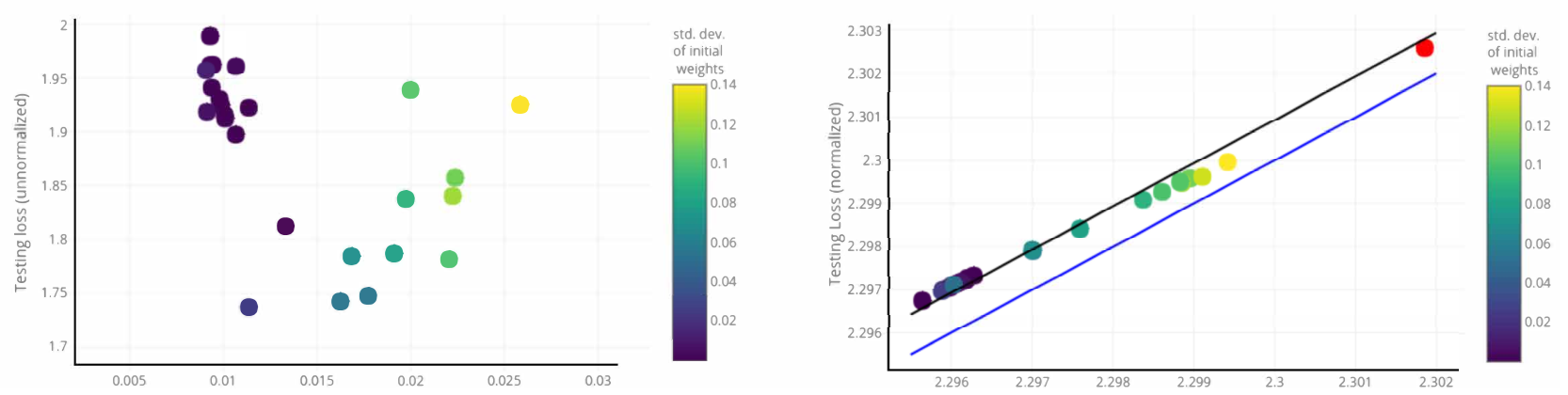
We’ve seen a lot of technical details regarding the dynamics of the parameters during training. But, how does this relates to the initial topic of generalization bounds? The general understanding is expecting that this preference for a particular solution poses a limitation on the class complexity thus explaining the generalization phenomena of deep neural networks. In fact, there is some empirical evidence that may favor the view generalization under normalized networks.

Furthermore, the concept of margin is already widely explored in the context of complexity measures (Antos et al. 2002, Bartlett et al. 2017) . Particularly, one of its main instruments is the estimate named Rademacher complexity. One example of such classical generalization bounds is:

$$R(h) \le R_n(h) + c_1\mathbb{R}_n(\mathcal{H}) + c_2\sqrt{\frac{ln(\frac{1}{\delta})}{2n}},$$

where $\mathbb{R}_n$ is the empirical estimate of the Rademacher complexity over the hypothesis class $\mathcal{H}$. However, making use of the homogeneity property $h = \rho\tilde{h}$ we arrive at:

$$R(\rho\tilde{h}) \le R_n(\rho\tilde{h}) + \rho\mathbb{R}_n(\widetilde{\mathcal{H}}) + c_2\sqrt{\frac{ln(\frac{1}{\delta})}{2n}},$$

the expectation is to decrease the class complexity while also controlling the generalization bound via $\rho$. However, as we already know, $\rho$ naturally increases throughout training, so even with techniques that promise to bound $\rho$ may not be enough to explain generalization in the current settings.

As of now, even though there’s no unified or undisputed explanation on the generalization of deep networks. Still, this is one of the most popular and prolific topics in theoretical machine learning. With this standing challenge come many competing explanations but also new directions and ingenious analyses, all of which could be used in demystifying deep networks as well as the new endeavors about to come.

References

• Shalev-Shwartz, S., & Ben-David, S. (2014). Understanding machine learning: From theory to algorithms. Cambridge university press.
• Neyshabur, B., Li, Z., Bhojanapalli, S., LeCun, Y., & Srebro, N. (2018). Towards understanding the role of over-parametrization in generalization of neural networks. arXiv preprint.
• Bishop, C. M. (1995). Training with noise is equivalent to Tikhonov regularization. Neural computation
• Goodfellow, I., Bengio, Y., Courville, A., & Bengio, Y. (2016). Deep learning. Cambridge: MIT press.
• Poggio, T., Liao, Q., & Banburski, A. (2020). Complexity control by gradient descent in deep networks. Nature communications.
• Banburski, A., Liao, Q., Miranda, B., Rosasco, L., Hidary, J., & Poggio, T. (2019). Theory III: Dynamics and Generalization in Deep Networks - a simple solution. arXiv preprint.
• Antos, A., Kégl, B., Linder, T., & Lugosi, G. (2002). Data-dependent margin-based generalization bounds for classification. Journal of Machine Learning Research.
• Bartlett, P. L., Foster, D. J., & Telgarsky, M. J. (2017). Spectrally-normalized margin bounds for neural networks. In Advances in neural information processing systems.